[Detection and Estimation] Estimation

On this page

• Detection and Estimation (Estimation part)
  • Lec 1. Introduction to statistical signal processing
  • Lec 2. Minimum Variance Unbiased(MVU) Estimation
    • Unbiased Estimators
    • Mean squared error(MSE) criterion
    • Minimum Variance Unbiased(MVU) Estimator
    • Existence of the MVU Estimator
    • Finding the MVU Estimator
  • Lec 3. Cramer-Rao Lower Bound (CRLB)
    • Cramer-Rao Lower Bound (CRLB)
    • Estimator Accuracy Considerations
    • Theorem: CRLB - Scalar Parameter
    • CRLB Proof (Appendix 3A)
    • General CRLB for Signals in WGN
    • Transformation of Parameters
    • Vector form of the CRLB
    • General Gaussian Case and Fisher Information
  • Lec 4.

Detection and Estimation (Estimation part)

GIST 황의석 교수님 [EC7204-01] Detection and Estimation 강의 정리 내용입니다.

---

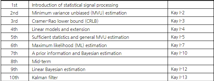
Lec 1. Introduction to statistical signal processing

- Goal of statistical signal processing

• Infer value of unknown state of nature based on noisy observations optimally

  

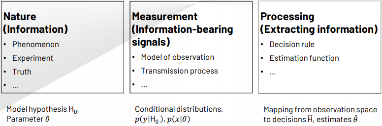
• deterministic에서는 \(P(x;\theta), P(y;\text{H}_0)\) . \(\theta\) 와 \(H_0\) 가 fixed 되어있는 문제

---

• Estimation은 Continuous 문제(SOH estimation), Detection은 Discrete 문제(Fault detection)

• Both Statistics and Machine Learning are concerned with the same question: How do we learn from data?

  Statistics emphasizes formal statistical inference,

  Machine Learning emphasizes high dimensional prediction problems

---

- Difference between detection and estimation …

• Estimation: Continuous set of hypotheses (almost always wrong - minimize error instead)

• Detection: Discrete set of hypotheses (right or wrong)

• Classical(deterministic): Hypotheses / parameters are fixed, non-random

• Bayesian: Hypotheses / parameters are treated as random variables with assumed priors (or a priori distributions)

  • Random parameter, random value, random state …

- Mathematical estimation problem

• Types of estimation

  • Classical estimation: parameters of interest are assumed to be deterministic.

  • Bayesian estimation: parameters are assumed to be random variables to exploit any prior knowledge(such as the average of Dow-Jones industrial average is in [2800, 3200])

    The data are described with joint pdf \(p(\mathbf{x}, \theta) = p(\mathbf{x} | \theta)p(\theta)\)

• Estimator and estimate

  • Estimator: a rule that assigns a value to \(\theta\) for each realization of \(\mathbf{x}\) (function of random variable \(\mathbf{x} \rightarrow\) random variable)

    • function \(g(·)\) , \(\hat{\theta} = g(x)\)

  • Estimate: the value of \(\theta\) obtained for a given realiztion of \(\mathbf{x}\)

- Assessing estimator performance

• Example of the DC level in noise

  • \(x[n] = A + w[n]\)

    

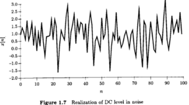
    \(A\) : unknown DC level

    \(w[n]\) : zero mean Gaussian process \(\sim \mathcal{N}(0,\sigma^2)\)

    \(N\) observations \(\{x[0],x[1],...,x[N-1]\}\)

  • Two candidate estimators (Sample mean vs. first sample value)

    • \(\hat{A}=\frac{1}{N}\sum^{N-1}_{n=0}x[n]\)

    • \(\check{A}= x[0]\)

• Statistical analysis

  • Mean

    • \(E(\hat{A}) = E(\frac{1}{N}\sum^{N-1}_{n=0}x[n]) = \frac{1}{n}\sum^{N-1}_{n=0}E(x[n])=A\)

    • \(E(\check{A}) = E(x[0]) = A\)

      둘다 unbiased

  • Variance

    • \(var(\hat{A}) = var(\frac{1}{N}\sum^{N-1}_{n=0}x[n]) = \frac{1}{N^2}\sum^{N-1}_{n=0}var(x[n])\)

      \(= \frac{1}{N^2}N\sigma^2 = \frac{\sigma^2}{N}\)

      N이 커지면 분산이 작아지는 모습

    • \(var(\check{A}) = var(x[0]) = \sigma^2\)

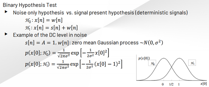
- Mathematical detection problem

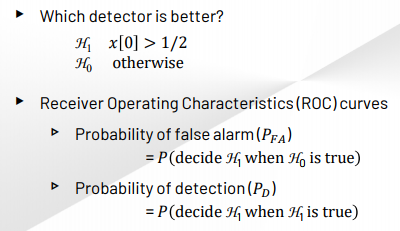
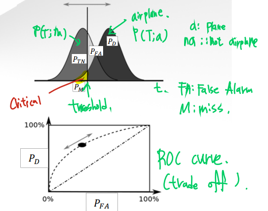
• Binary Hypothesis Test

  

- Assessing detector pereformance

• 

  

Review

• Parameter: We wish to estimate the unknown parameter \(\theta\) from observation(s) \(x\). These can be vectors \(\mathbf{\theta} = [\theta_0, \theta_1, ..., \theta_p]^T\) and \(\mathbf{x} = [x[0], x[1], ..., x[N-1]]^T\) or scalars.

• Parameterized PDF: the unknown parameter \(\theta\) is to be estimated. \(\theta\) parametrizes the PDF of the received data \(p(x;\theta)\).

  When dealing with Bayesian estimators, the notation \(p(x|\theta)\) will be used to highlight the fact that \(\theta\) is a random variable.

  Mutual information 관련.. \(\theta\)가 정보가 있으면 \(p(x|\theta)\)는 \(p(x)\)보다 나을 것

• Estimator: a rule that assigns a value \(\hat{\theta}\) to \(\theta\) for each realization of \(x\).

• Estimate: the value of \(\theta\) obtained for a given realization of \(x\). \(\hat{\theta}\) will be used for the estimate, while \(\theta\) will represent the true value of the unknown parameter.

• Mean and variance of the estimator: \(E(\hat{\theta})\) and \(var(\hat{\theta}) = E[(\hat{\theta}-E(\hat{\theta}))^2]\).

  Expectations are taken over \(x\) (meaning \(\hat{\theta}\) is random, not \(\theta\).)

\(x\): 항상 랜덤

\(\theta\): 항상 랜덤은 아니지만 랜덤이 될 수 있다. (\(\hat{\theta}\): random)

• Classical: fixed (;)

• Bayesian: conditional (|)

---

Lec 2. Minimum Variance Unbiased(MVU) Estimation

Unbiased Estimators

• An estimator \(\hat{\theta}\) is called unbiased, if \(E(\hat{\theta}) = \theta\) for all possible \(\theta\).

  \(\hat{\theta} = g(x) \Rightarrow E(\hat{\theta}) = \int g(x)p(x;\theta)dx = \theta\)

• If \(E(\hat{\theta} \neq \theta)\), the bias is \(b(\theta) = E(\hat{\theta}) - \theta\)

  (Expectation is taken with respect to \(x\) or \(p(x;\theta)\))

• \(E(\hat{\theta}) = \theta\) may hold for some values of \(\theta\) for biased estimators, i.e., modified sample mean estimator

  \(\check{A} = \frac{1}{2N} \sum_{n=0}^{N-1} x[n] \quad \Rightarrow \quad E(\check{A}) = \frac{1}{2}A \begin{cases} = A \text{ if } A = 0 \\ \neq A \text{ if } A \neq 0 \end{cases} \rightarrow\) biased

• Unbiased estimator is not necessarily a good estimator;

  but a biased estimator is a poor estimator.

- biased estimator \(E[\hat{\sigma}^2]\)

• 모평균 \(\mu\), 모분산 \(\sigma^2\): Unknown

• \(E[x[n]] = \mu\)

  \(\text{Var}[x[n]] = \sigma^2 = E[x^2[n]] - E^2[x[n]]\)

  \(E[x^2[n]] = \sigma^2 + \mu^2 \cdots (*)\)

• \(\bar{x} = \frac{1}{N}\sum^{N-1}_{n=0} x[n]\) (sample mean)

  \(E[\bar{x}] = \mu \leftarrow\) unbiased

  \(\text{Var}[\bar{x}] = \frac{\sigma^2}{N} = E[\bar{x}^2] - \mu^2\)

  \(\rightarrow E[\bar{x}^2] = \frac{\sigma^2}{N} + \mu^2 \cdots (**)\)

• \(\hat{\sigma}^2 = \frac{1}{N} \sum^{N-1}_{n=0}(x[n] - \bar{x})^2\)

  \(E[\hat{\sigma}^2] = \frac{1}{N} E[\sum^{N-1}_{n=0}(x^2[n])-2\bar{x}\sum^{N-1}_{n=0}x[n] + N \bar{x}^2]\)

  \(\quad\quad\quad = \frac{1}{N}E[\sum x^2[n] - N\bar{x}^2]\)

  \(\quad\quad\quad = \frac{1}{N}(\sum(E[x^2[n]]) - N E[\bar{x}^2])\) 여기서 (*) 과 (**)에 의해

  \(\quad\quad\quad = \frac{1}{N}(N(\sigma^2 + \mu^2) - N(\frac{\sigma^2}{N} + \mu^2))\)

  \(\quad\quad\quad = \frac{1}{N}(N\sigma^2 - \sigma^2)\)

  \(\quad\quad\quad = \frac{N-1}{N}\sigma^2 \cdots\) “biased estimator”

• 이에 따라, 표본 분산을 unbiased estimator로 만들기 위해선

  \(\hat{\sigma}^2 = \frac{1}{N} \sum^{N-1}_{n=0}(x[n] - \bar{x})^2\) 가 아닌

  \(\hat{\sigma}^2 = \frac{1}{N-1} \sum^{N-1}_{n=0}(x[n] - \bar{x})^2\) 을 사용하여야 한다!

Mean squared error(MSE) criterion

• MSE Criterion

  \(\text{mse}(\hat{\theta}) = E\left[(\hat{\theta} - \theta)^2\right]\)

  \(\quad\quad\quad = E\left[\left((\hat{\theta} - E(\hat{\theta})) + (E(\hat{\theta}) - \theta)\right)^2\right]\)

  \(\quad\quad\quad = \text{var}(\hat{\theta}) + \left[E(\hat{\theta}) - \theta\right]^2\)

  \(\quad\quad\quad = \text{var}(\hat{\theta}) + b^2(\theta)\)

• Note that, in many cases, minimum MSE criterion leads to unrealizable estimator, which cannot be written solely as a function of the data, i.e.,

  여기선 Sample Mean으로 예시를 들었다.

  \(\check{A} = a \frac{1}{N} \sum_{n=0}^{N-1} x[n]\) where \(a\) is chosen to minimize MSE.

  Then, \(E(\check{A}) = aA, \quad var(\check{A}) = \frac{a^2 \sigma^2}{N} \quad \Rightarrow \quad \text{mse}(\check{A}) = \frac{a^2 \sigma^2}{N} + (a-1)^2 A^2\)

  MSE를 최소화하기 위해 미분을 해보면 \(\frac{d \text{mse}(\check{A})}{d a} = \frac{2a \sigma^2}{N} + 2(a-1) A^2 = 0\) (optimize)

  \(\Rightarrow a_{opt} = \frac{A^2}{A^2 + \frac{\sigma^2}{N}} \quad \text{(unrealizable, a function of unknown A)}\) A를 모르기에 사용 불가

  하지만 만약 \(\text{mse}(\check{A}) = \frac{a^2 \sigma^2}{N} + (a-1)^2 A^2\) 에서 bias term인 \((a-1)^2 A^2\) 가 0이 된다면?(unbiased 라면) → 최적의 a값을 찾는 것이 가능할 것!

Minimum Variance Unbiased(MVU) Estimator

• Any criterion that depends on the bias is likely to be unrealizable → Practically minimum MSE estimator needs to be abandoned Minimum variance unbiased(MVU) estimator

  • Alternatively, constrain the bias to be zero

  • Find the estimator which minimizes the variance (minimizing the MSE as well for unbiased case)

  \(\text{mse}(\hat{\theta}) = \text{var}(\hat{\theta}) + b^2(\theta)\)

  \(\quad\quad\quad= \text{var}(\hat{\theta})\)

  → Minimum variance unbiased (MVU) estimator

Existence of the MVU Estimator

• An unbiased estimator with minimum variance for all \(\theta\)

• Examples

  

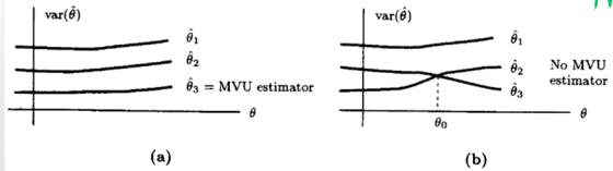
• In general, the MVUE estimator does not always exist!

Finding the MVU Estimator

There is no general framework to find MVU estimator even if it exists.

Possible approaches:

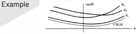
1. Determine the Cramer-Rao lower bound (CRLB) and check if some estimator satisfies it (challenge)

2. Apply the Rao-Blackwell-Lehmann-Scheffe (RBLS) theorem (challenge)

3. Fine unbiased linear estimator with minimum variance (best linear unbiased estimator, BLUE)

   

---

Lec 3. Cramer-Rao Lower Bound (CRLB)

Cramer-Rao Lower Bound (CRLB)

• The CRLB give a lower bound on the variance of any unbiased estimator. (biased의 경우는 알 수 없다!)

• Does not guarantee bound can be obtained.

• 만약 unbiased estimator의 variance가 CRLB라면 그 estimator는 MVUE.

Estimator Accuracy Considerations

• All information is observed data and underlying PDF → Estimation accuracy depends directly on the PDF.

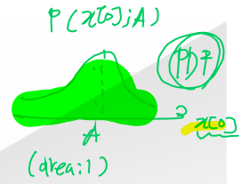
• PDF: 값이 나타날 가능성. 파라미터는 고정! 영역의 넓이는 1

• Likelihood (우도): 주어진 데이터가 특정 파라미터 값에 의해 생성되었을 가능성을 나타낸다.

  Likelihood는 확률 자체는 아니며, 데이터가 이미 주어졌을 때 그 데이터를 설명하는 파라미터의 값이 얼마나 그럴듯한지를 측정한다.

  즉, 파라미터를 고정하지 않고 데이터를 고정한 상태에서 파라미터를 추정하는 과정에서 사용된다.

  데이터를 기반으로 가장 그럴듯한 파라미터 값을 찾기 위한 것

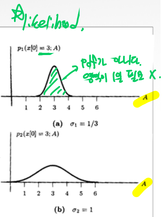
• 영역의 넓이는 1일 필요가 없다!

• 직관적으로 likelihood function의 “sharpness”가 측정의 정확도를 결정한다는 것을 알 수 있다.

• likelihood function이 다음과 같다고 하면,

  \[p(x[0];A) = \frac{1}{\sqrt{2\pi\sigma^2}}\text{exp}[-\frac{1}{2\sigma^2}(x[0]-A)^2]\]

  log-likelihood function은 다음과 같고

  \[\text{ln}\ p(x[0];A) = -\text{ln}\sqrt{2\pi\sigma^2}-\frac{1}{2\sigma^2}(x[0]-A)^2\]

  A에 대해 두번 미분해주고 마이너스를 붙여주면

  \[-\frac{\partial ^2 \text{ln}\ p(x[0];A)}{\partial A^2} = \frac{1}{\sigma^2}, \quad \quad \text{var}(\hat{A}) = \sigma^2 = \frac{1}{-\frac{\partial ^2 \text{ln}\ p(x[0];A)}{\partial A^2}}\]

  More appropriate measure is average curvature(곡률, (2차미분 값)), \(-E[\frac{\partial ^2 \text{ln}\ p(x[0];A)}{\partial A^2}]\)

  (In general, the \(2^{\text{nd}}\) derivative will depend on \(x[0] \rightarrow\) the likelihood function is a R.V.)

Theorem: CRLB - Scalar Parameter

• Let \(p(\mathbf{x}; \theta)\) satisfy the “regularity” condition

  \[E_\mathbf{x}[\frac{\partial\text{ln}\ p(\mathbf{x}; \theta)}{\partial \theta}] = 0\quad \text{for all}\ \theta\]

  Then, the variance of any unbiased estimator \(\hat{\theta}\) must satisfy

  \[\text{var}(\hat{\theta}) \ge \frac{1}{-E_\mathbf{x}[\frac{\partial^2\text{ln}\ p(\mathbf{x}; \theta)}{\partial \theta^2}]} = \frac{1}{E_\mathbf{x}[(\frac{\partial\text{ln}\ p(\mathbf{x}; \theta)}{\partial \theta})^2]}\]

  where the derivative is evaluated at the true value \(\theta\) and the expectation is taken w.r.t. \(p(\mathbf{x};\theta).\)

  여기서 세번째 텀에서 - 가 사라지는 이유는, 두번째 텀에서 - 가 붙는 이유를 생각해보면 된다.

  두번째 텀에서 마이너스가 붙는 이유는 값을 양수로 만들어주기 위함이고, 세번째 텀은 일차 미분의 제곱이므로 자연스럽게 양수이다. 따라서 - 가 사라지게 된다.

  Furthermore, an unbiased estimator may be found that attains the bound for all \(\theta\) if and only if

  \[\frac{\partial\ \text{ln}\ p(\mathbf{x}; \theta)}{\partial \theta} = I(\theta)(g(\mathbf{x})-\theta)\]

  for some functions \(g()\) and \(I\). That estimator, which is the MVUE, is \(\hat{\theta} = g(\mathbf{x})\), and the minimum variance is \(\frac{1}{I(\theta)}\)

• Fisher Information: 추정 정확도를 측정하는 방법. 우도 함수의 곡률이 크면 추정량의 분산이 작고, 더 정확한 추정을 할 수 있음을 의미

• 정칙성 조건(Regularity Conditions): CRLB가 성립하기 위한 조건으로, 특정 미분 가능성 조건을 만족해야 한다.

CRLB Proof (Appendix 3A)

• CRLB for scalar parameter \(\alpha = g(\theta)\) where the PDF is parameterized with \(\theta\).

  Consider unbiased estimator \(\hat{\alpha}\), i.e.,

  \[E(\hat{\alpha}) = \int \hat{\alpha} p (\mathbf{x}; \theta)d \mathbf{x} = \alpha = g(\theta) \quad \cdots \quad(*)\]

  Regularity condition (holds if the order of differentiation and integration may be interchanged)

  \[E[\frac{\partial \text{ln}\ p(\mathbf{x}; \theta)}{\partial \theta}] = \int \frac{\partial \text{ln}\ p(\mathbf{x}; \theta)}{\partial \theta} p(\mathbf{x}; \theta) d \mathbf{x} = 0\]

  Differentiating both sides of \((*)\)

  \[\int \hat{\alpha} \frac{\partial p (\mathbf{x}; \theta)}{\partial \theta}d \mathbf{x} = \frac{\partial g(\theta)}{\partial \theta}\]

  여기서 로그함수에 대한 미분식을 이용하면 \((\frac{\partial}{\partial \theta} \text{ln}\ p(x; \theta) = \frac{1}{p(x;\theta)}\frac{\partial}{\partial \theta} p(x;\theta))\)

  \[\Rightarrow \int \hat{\alpha} \frac{\partial \text{ln} p(\mathbf{x};\theta)}{\partial \theta} p(\mathbf{x}; \theta) d \mathbf{x} = \frac{\partial g(\theta)}{\partial \theta}\]

  보면 위의 Expectation 식과 동일함을 알 수 있다.

  By using regularity condition,

  \[\int (\hat{\alpha} - \alpha) \frac{\partial \text{ln}\ p(\mathbf{x};\theta)d\mathbf{x}}{\partial \theta}p(\mathbf{x}; \theta) d\mathbf{x} = \frac{\partial g(\theta)}{\partial \theta}\]

  By using Cauchy-Schwarz inequality, (코시 슈바르츠 부등식은 아래에 서술)

  \[(\frac{\partial g(\theta)}{\partial \theta})^2 \le \int (\hat{\alpha} - \alpha)^2 p (\mathbf{x};\theta) d\mathbf{x} \int (\frac{\partial \text{ln}\ p(\mathbf{x}; \theta)}{\partial \theta})^2 p(\mathbf{x}; \theta) d \mathbf{x}\]

  \[\rightarrow \text{var}(\hat{\alpha}) \ge \frac{(\frac{\partial g(\theta)}{\partial \theta})^2}{E[(\frac{\partial \text{ln}\ p(\mathbf{x}; \theta)}{\partial \theta})^2]}\]

• By differentiating the regularity condition,

  \[\frac{\partial}{\partial \theta} \int \frac{\partial \text{ln}\ p(\mathbf{x}; \theta)}{\partial \theta} p (\mathbf{x}; \theta) d \mathbf{x} = 0\]

  \[\int [\frac{\partial^2 \text{ln} p (\mathbf{x};\theta)}{\partial \theta^2} p (\mathbf{x}; \theta) + \frac{\partial \text{ln} p (\mathbf{x}; \theta)}{\partial \theta} \frac{\partial p(\mathbf{x}; \theta)}{\partial \theta}]d \mathbf{x} = 0\]

  \[- E[\frac{\partial ^2 \text{ln} p(\mathbf{x}; \theta)}{\partial \theta^2}] = \int \frac{\partial \text{ln} p(\mathbf{x};\theta)}{\partial \theta} \frac{\partial \text{ln} p (\mathbf{x}; \theta)}{\partial \theta} p (\mathbf{x};\theta)d \mathbf{x} = E[(\frac{\partial \text{ln} p (\mathbf{x}; \theta)}{\partial \theta})^2]\]

  \[\rightarrow \text{var}(\hat{\alpha}) \ge \frac{(\frac{\partial g(\theta)}{\partial \theta})^2}{E[(\frac{\partial \text{ln} p(\mathbf{x}; \theta)}{\partial \theta})^2]} = \frac{(\frac{\partial g(\theta)}{\partial \theta})^2}{-E[\frac{\partial^2 \text{ln} p(\mathbf{x}; \theta)}{\partial \theta^2}]}\]

• If \(\alpha = g(\theta) = \theta\),

  \[\text{var}(\hat{\theta}) \ge \frac{1}{-E[\frac{\partial^2 \text{ln} p (\mathbf{x}; \theta)}{\partial \theta^2}]} = \frac{1}{E[(\frac{\partial \text{ln} p(\mathbf{x}; \theta)}{\partial \theta})^2]}\]

  Condition for equality :

  \[\frac{\partial \text{ln} p (\mathbf{x}; \theta)}{\partial \theta} = \frac{1}{c}(\hat{\alpha}- \alpha)\]

• If \(\alpha = g(\theta) = \theta\),

  \[\frac{\partial \text{ln} p (\mathbf{x}; \theta)}{\partial \theta} = \frac{1}{c}(\hat{\theta}- \theta)\]

  To determine \(c(\theta)\),

  \[\frac{\partial^2 \text{ln} p (\mathbf{x}; \theta)}{\partial \theta^2} = - \frac{1}{c(\theta)} + \frac{\partial(\frac{1}{c(\theta)})}{\partial \theta}(\hat{\theta} - \theta)\]

  \[- E [\frac{\partial^2 \text{ln} p(\mathbf{x}; \theta)}{\partial \theta^2}] = \frac{1}{c(\theta)} = I(\theta)\]

- Cauchy-Schwarz Inequality?

\[[\int w(\mathbf{x}) g(\mathbf{x}) h(\mathbf{x}) d \mathbf{x}]^2 \le \int w(\mathbf{x}) g^2 (\mathbf{x}) d \mathbf{x} \int w(\mathbf{x}) h^2(\mathbf{x}) d \mathbf{x}\]

• Arbitary function \(g(\mathbf{x})\) and \(h(\mathbf{x})\), while \(w(\mathbf{x}) \ge 0\) for all \(\mathbf{x}\).

  Equality holds in and only if

  \[g(\mathbf{x}) = c\ h(\mathbf{x})\]

General CRLB for Signals in WGN

Transformation of Parameters

Vector form of the CRLB

General Gaussian Case and Fisher Information

---

Lec 4.