Numpy_Tutorial
넘파이 튜토리얼


import numpy as np
- NumPy’s main object = the homogeneous multidimensional array.
- In NumPy dimensions are called axes.
1차원

[1, 2, 1]

2차원

[[ 1., 0., 0.],
 [ 0., 1., 2.]]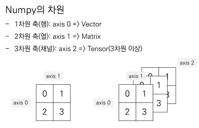
- NumPy’s array class is called ndarray.
- numpy.array is not the same as the Standard Python Library class array.
- 파이썬의 array는 1차원만을 다룬다.
- The more important attributes of an ndarray object are:
-
ndarray.ndim: 넘파이의 차원 -
ndarray.shape: 넘파이의 모양 (n, m) -
ndarray.size: This is equal to the product of the elements of shape. (n*m) -
ndarray.dtype: array안 요소의 타입 -
ndarray.itemsize: array안 요소들의 사이즈(bytes) -
ndarray.data: Normally, we won’t need to use this attribute because we will access the elements in an array using indexing facilities.
-
An example
>>> import numpy as np
>>> a = np.arange(15).reshape(3, 5)
>>> a
array([[ 0,  1,  2,  3,  4],
       [ 5,  6,  7,  8,  9],
       [10, 11, 12, 13, 14]])

>>> a.shape
(3, 5)

>>> a.ndim
2

>>> a.dtype.name
'int64'

>>> a.itemsize
8

>>> a.size
15

>>> type(a)
<type 'numpy.ndarray'>

>>> b = np.array([6, 7, 8])
>>> b
array([6, 7, 8])

>>> type(b)
<type 'numpy.ndarray'>
you can create an array from a regular Python list or tuple using the array function.
>>> a = np.array([2,3,4])
>>> a
array([2, 3, 4])
2차원 array
>>> b = np.array([(1.5,2,3), (4,5,6)])
>>> b
array([[ 1.5,  2. ,  3. ],
       [ 4. ,  5. ,  6. ]])
The function zeros creates an array full of zeros,
>>> np.zeros( (3,4) )
array([[ 0.,  0.,  0.,  0.],
       [ 0.,  0.,  0.,  0.],
       [ 0.,  0.,  0.,  0.]])

>>> np.ones( (2,3,4), dtype=np.int16 )                # dtype can also be specified
array([[[ 1, 1, 1, 1],
        [ 1, 1, 1, 1],
        [ 1, 1, 1, 1]],
       [[ 1, 1, 1, 1],
        [ 1, 1, 1, 1],
        [ 1, 1, 1, 1]]], dtype=int16)
To create sequences of numbers, NumPy provides a function analogous to range that returns arrays instead of lists.
>>> np.arange( 10, 30, 5 )
array([10, 15, 20, 25])
>>> np.arange( 0, 2, 0.3 )                 # it accepts float arguments
array([ 0. ,  0.3,  0.6,  0.9,  1.2,  1.5,  1.8])


>>> np.linspace( 0, 2, 9 )                 # 9 numbers from 0 to 2
array([ 0.  ,  0.25,  0.5 ,  0.75,  1.  ,  1.25,  1.5 ,  1.75,  2.  ])
other method
array, zeros, zeros_like, ones, ones_like, empty, empty_like, arange, linspace, numpy.random.rand, numpy.random.randn, fromfunction, fromfile1차원은 행으로, 2,3 차원은 행렬로 표현된다.
>>> a = np.arange(6)                         # 1d array
>>> print(a)
[0 1 2 3 4 5]

>>> b = np.arange(12).reshape(4,3)           # 2d array
>>> print(b)
[[ 0  1  2]
 [ 3  4  5]
 [ 6  7  8]
 [ 9 10 11]]

>>> c = np.arange(24).reshape(2,3,4)         # 3d array
>>> print(c)
[[[ 0  1  2  3]
  [ 4  5  6  7]
  [ 8  9 10 11]]
 [[12 13 14 15]
  [16 17 18 19]
  [20 21 22 23]]]
>>> a = np.array( [20,30,40,50] )
>>> b = np.arange( 4 )
>>> b
array([0, 1, 2, 3])
>>> c = a-b
>>> c
array([20, 29, 38, 47])
>>> b**2
array([0, 1, 4, 9])
>>> 10*np.sin(a)
array([ 9.12945251, -9.88031624,  7.4511316 , -2.62374854])
>>> a<35
array([ True, True, False, False])
*는 각각의 요소끼리 곱하고 @, dot은 행렬곱을 한다.
>>> A = np.array( [[1,1],
...             [0,1]] )
>>> B = np.array( [[2,0],
...             [3,4]] )
>>> A * B                       # elementwise product
array([[2, 0],
       [0, 4]])
>>> A @ B                       # matrix product
array([[5, 4],
       [3, 4]])
>>> A.dot(B)                    # another matrix product
array([[5, 4],
       [3, 4]])
+= , *= 연산
> >> a = np.ones((2,3), dtype=int)
>>> b = np.random.random((2,3))

>>> a *= 3
>>> a
array([[3, 3, 3],
       [3, 3, 3]])

>>> b += a
>>> b
array([[ 3.417022  ,  3.72032449,  3.00011437],
       [ 3.30233257,  3.14675589,  3.09233859]])

>>> a += b                  # b is not automatically converted to integer type
Traceback (most recent call last):...TypeError: Cannot cast ufunc add output from dtype('float64') to dtype('int64') with casting rule 'same_kind'
전체합, 최솟값, 최댓값 등을 구할때는 ndarray 자체 메소드를 사용하여야한다.
>>> a = np.random.random((2,3))
>>> a
array([[ 0.18626021,  0.34556073,  0.39676747],
       [ 0.53881673,  0.41919451,  0.6852195 ]])
>>> a.sum()
2.5718191614547998
>>> a.min()
0.1862602113776709
>>> a.max()
0.6852195003967595
연산들은 전체를 기준으로 하지만, axis를 추가해주면 각 행이나 열마다 함수를 적용할 수 있다.
>>> b
array([[ 0,  1,  2,  3],
       [ 4,  5,  6,  7],
       [ 8,  9, 10, 11]])
>>>
>>> b.sum(axis=0)                            # sum of each column
array([12, 15, 18, 21])
>>>
>>> b.min(axis=1)                            # min of each row
array([0, 4, 8])
>>>
>>> b.cumsum(axis=1)                         # cumulative sum along each row 누적합
array([[ 0,  1,  3,  6],
       [ 4,  9, 15, 22],
       [ 8, 17, 27, 38]])
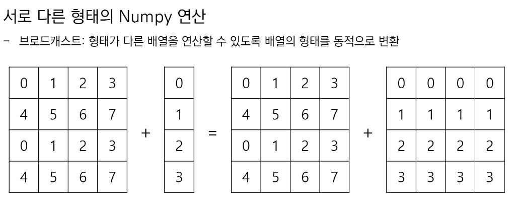
- 서로 다른 형태의 Numpy 연산
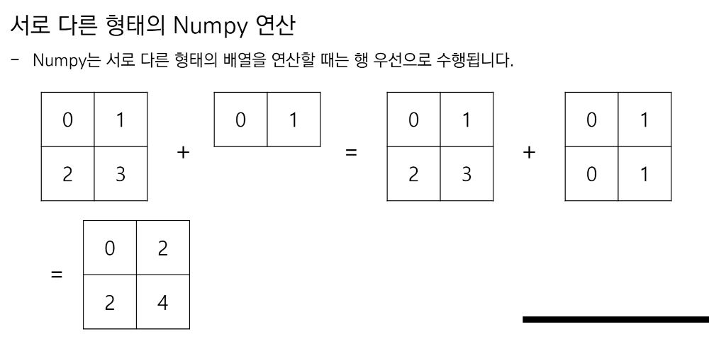
array1 = np.arange(4).reshape(2,2)
array2 = np.arange(2)
array3 = array1 + array2
print(array3)
- 브로드캐스트
- 마스킹 연산
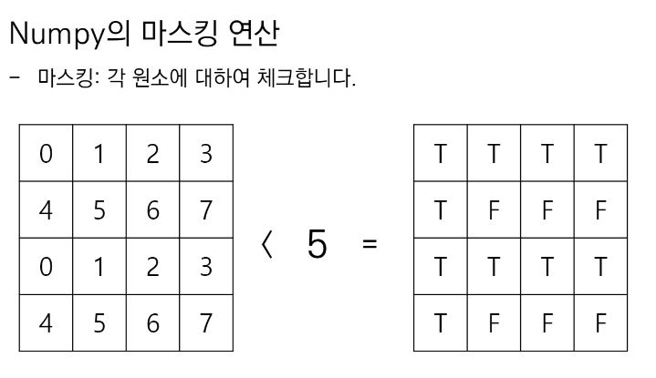
Numpy 원소의 값을 조건에 따라 바꿀 때 다음과 같이한다.
반복문을 이용할 때보다 매우 빠르게 동작한다.
대체로 이미지 처리(Image Processing)에서 자주 활용된다.
array1 = np.arange(16).reshape(4,4)
print(array1)

array2 = array1 < 10
print(array2)

array1[array2] = 100
print(array1)
Universal Functions
- NumPy provides familiar mathematical functions such as sin, cos, and exp. In NumPy, these are called “universal functions”(ufunc).
>>> B = np.arange(3)
>>> B
array([0, 1, 2])
>>> np.exp(B)
array([ 1.        ,  2.71828183,  7.3890561 ])
>>> np.sqrt(B)
array([ 0.        ,  1.        ,  1.41421356])
>>> C = np.array([2., -1., 4.])
>>> np.add(B, C)
array([ 2.,  0.,  6.])
other method
all, any, apply_along_axis, argmax, argmin, argsort, average, bincount, ceil, clip, conj, corrcoef, cov, cross, cumprod, cumsum, diff, dot, floor, inner, inv, lexsort, max, maximum, mean, median, min, minimum, nonzero, outer, prod, re, round, sort, std, sum, trace, transpose, var, vdot, vectorize, where- 1차원 array는 파이썬의 리스트와 같이 인덱싱, 슬라이싱을 할 수 있다,
-
Multidimensional arrays can have one index per axis. These indices are given in a tuple separated by commas
반점을 사이에 둔 튜플 필요
> >> def f(x,y):...     return 10*x+y...
> >> b = np.fromfunction(f,(5,4),dtype=int)
>>> b
array([[ 0,  1,  2,  3],
     [10, 11, 12, 13],
     [20, 21, 22, 23],
     [30, 31, 32, 33],
     [40, 41, 42, 43]])
>>> b[2,3]
23
>>> b[0:5, 1]                       # each row in the second column of barray([ 1, 11, 21, 31, 41])
> >> b[ :,1]                        # equivalent to the previous examplearray([ 1, 11, 21, 31, 41])
> >> b[1:3, : ]                      # each column in the second and third row of barray([[10, 11, 12, 13],[20, 21, 22, 23]])
Iterating over multidimensional arrays is done with respect to the first axis:
> >> for row in b:print(row)
[0 1 2 3]
[10 11 12 13]
[20 21 22 23]
[30 31 32 33]
[40 41 42 43]
However, if one wants to perform an operation on each element in the array, one can use the flat attribute which is an iterator over all the elements of the array:
> >> for element in b.flat:print(element)
0
1
2
3
10
11
12
13
20
21
22
23
30
31
32
33
40
41
42
43
other method
Indexing, Indexing (reference), newaxis, ndenumerate, indices- 모양을 바꾸는 3가지 방법
ravel(),reshape(),T. 하지만 원래의 array는 바뀌지않는다!
>>> a.shape
(3, 4)

>>> a.ravel()  # returns the array, flattened
array([ 2.,  8.,  0.,  6.,  4.,  5.,  1.,  1.,  8.,  9.,  3.,  6.])

>>> a.reshape(6,2)  # returns the array with a modified shape
array([[ 2.,  8.],
       [ 0.,  6.],
       [ 4.,  5.],
       [ 1.,  1.],
       [ 8.,  9.],
       [ 3.,  6.]])

>>> a.T  # returns the array, transposed
array([[ 2.,  4.,  8.],
       [ 8.,  5.,  9.],
       [ 0.,  1.,  3.],
       [ 6.,  1.,  6.]])

>>> a.T.shape
(4, 3)

>>> a.shape
(3, 4)
- 이번엔 원래의 array를 바꾸는 메소드
resize>>> a array([[ 2., 8., 0., 6.], [ 4., 5., 1., 1.], [ 8., 9., 3., 6.]]) >>> a.resize((2,6)) >>> a array([[ 2., 8., 0., 6., 4., 5.], [ 1., 1., 8., 9., 3., 6.]])
- 행이나 열로 여러개의 array를 쌓을 수 있다.
>>> a = np.floor(10*np.random.random((2,2)))
>>> a
array([[ 8.,  8.],
     [ 0.,  0.]])
>>> b = np.floor(10*np.random.random((2,2)))
>>> b
array([[ 1.,  8.],
     [ 0.,  4.]])
>>> np.vstack((a,b))
array([[ 8.,  8.],
     [ 0.,  0.],
     [ 1.,  8.],
     [ 0.,  4.]])
>>> np.hstack((a,b))
array([[ 8.,  8.,  1.,  8.],
     [ 0.,  0.,  0.,  4.]])
- 가로축으로 합치고 싶을 때
array1 = np.array([1,2,3])
array2 = np.array([4,5,6])
array3 = np.concatenate([array1, array2])

print(array3.shape)
print(array3)
- 세로축으로 합치고 싶을 때
array1 = np.arange(4).reshape(1,4)
array2 = np.arange(8).reshape(2,4)

print(array1)
print(array2)

array3 = np.concatenate([array1, array2], axis = 0) # axis = 0 이 추가됨!
print(array3)
other method
hstack, vstack, column_stack, concatenate, c_, r_- 각 행을 원하는 갯수로 나누어준다.
>>> a = np.floor(10*np.random.random((2,12)))
>>> a
array([[ 9.,  5.,  6.,  3.,  6.,  8.,  0.,  7.,  9.,  7.,  2.,  7.],
       [ 1.,  4.,  9.,  2.,  2.,  1.,  0.,  6.,  2.,  2.,  4.,  0.]])
>>> np.hsplit(a,3)   # Split a into 3
[array([[ 9.,  5.,  6.,  3.],
       [ 1.,  4.,  9.,  2.]]), array([[ 6.,  8.,  0.,  7.],
       [ 2.,  1.,  0.,  6.]]), array([[ 9.,  7.,  2.,  7.],
       [ 2.,  2.,  4.,  0.]])]
-
split이용
import numpy as np
array = np.arange(8).reshape(2, 4)
left, right = np.split(array, [2], axis=1) # array에서 3번째열을 기준으로 나눈다.
print(left.shape)
print(right.shape)
print(array)
print(left)
- 복사와 관련해서 초보자들이 실수하는 3가지
>>> a = np.arange(12)
>>> b = a            # no new object is created
>>> b is a           # a and b are two names for the same ndarray object
True
>>> b.shape = 3,4    # changes the shape of a
>>> a.shape
(3, 4)
b라는 새로운 객체가 생긴게 아니라 b가 곧 a
-
View메서드는 동일한 데이터를 보는 새 배열 개체를 만든다.>>> c = a.view() >>> c is a False >>> c.base is a # c is a view of the data owned by a True >>> c.flags.owndata False >>> >>> c.shape = 2,6 # a's shape doesn't change >>> a.shape (3, 4) >>> c[0,4] = 1234 # a's data changes >>> a array([[ 0, 1, 2, 3], [1234, 5, 6, 7], [ 8, 9, 10, 11]
- 배열을 슬라이싱하면 배열의 뷰가 반환된다.
> >> s = a[ :, 1:3]     # spaces added for clarity; could also be written "s = a[:,1:3]"> >> s[:] = 10           # s[:] is a view of s. Note the difference between s=10 and s[:]=10>>> a
array([[   0,   10,   10,    3],
     [1234,   10,   10,    7],
     [   8,   10,   10,   11]])
-
copy메서드는 배열과 그 데이터의 완전한 복사를 만들어준다.
>>> d = a.copy()                          # a new array object with new data is created
>>> d is a
False
>>> d.base is a                           # d doesn't share anything with a
False
>>> d[0,0] = 9999
>>> a
array([[   0,   10,   10,    3],
       [1234,   10,   10,    7],
       [   8,   10,   10,   11]])
>>> a = np.arange(12)**2                       # the first 12 square numbers
>>> i = np.array( [ 1,1,3,8,5 ] )              # an array of indices
>>> a[i]                                       # the elements of a at the positions i
array([ 1,  1,  9, 64, 25])
>>>
>>> j = np.array( [ [ 3, 4], [ 9, 7 ] ] )      # a bidimensional array of indices
>>> a[j]                                       # the same shape as j
array([[ 9, 16],
       [81, 49]])
+