CS231n_CNN for Visual Recognition
Stanford University CS231n


- Image Classification
- Linear Classification
- Optimization
- Backprop
- Neural Network - 1
- Neural Network - 2
- Neural Network - 3
- CNN
- Spatial Localization and Detection
- CNNs in practice
- Segmentaion
-
Image Classification: 우리에겐 라벨링된 이미지의 트레이닝 셋이 주어지고, 테스트셋의 라벨을 예측해야한다. 흔히 Accuracy로 평가한다.(예측된 이미지의 정답비율)
-
We introduced the k-Nearest Neighbor Classifier, 이는 트레이닝 셋에서 가장 가까운 이미지에 기반하여 예측을 한다.
-
우리는 validation set을 (데이터가 작을 때에는 cross-validation을) 사용하여 거리와 k의 값을 선택하는 즉 하이퍼파라미터를 튜닝하는것을 보았다.
-
최고의 하이퍼파라미터가 선택되면, 분류기는 테스트셋에서 평가되고 해당 데이터에서 kNN의 성능이라고 보고된다.
-
Nearest Neighbor 분류기는 CIFAR-10 데이터셋에서 약 40% 정도의 정확도를 보이는 것을 확인하였다. 이 방법은 구현이 매우 간단하지만, 학습 데이터셋 전체를 메모리에 저장해야 하고, 새로운 테스트 이미지를 분류하고 평가할 때 계산량이 매우 많다.
-
단순히 픽셀 값들의 L1이나 L2 거리는 이미지의 클래스보다 배경이나 이미지의 전체적인 색깔 분포 등에 더 큰 영향을 받기 때문에 이미지 분류 문제에 있어서 충분하지 못하다는 점을 보았다.
-
We defined a score function from image pixels to class scores (in this section, a linear function that depends on weights W and biases b).
-
Unlike kNN classifier, the advantage of this parametric approach is that once we learn the parameters we can discard the training data. Additionally, the prediction for a new test image is fast since it requires a single matrix multiplication with W, not an exhaustive comparison to every single training example.
-
We introduced the bias trick, which allows us to fold the bias vector into the weight matrix for convenience of only having to keep track of one parameter matrix. 하나의 매개변수 행렬만 추적해야 하는 편의를 위해 편향 벡터를 가중치 행렬로 접을 수 있는 편향 트릭을 도입했습니다 .
-
We defined a loss function (we introduced two commonly used losses for linear classifiers: the SVM and the Softmax) that measures how compatible a given set of parameters is with respect to the ground truth labels in the training dataset. We also saw that the loss function was defined in such way that making good predictions on the training data is equivalent to having a small loss.
-
We developed the intuition of the loss function as a high-dimensional optimization landscape in which we are trying to reach the bottom. The working analogy we developed was that of a blindfolded hiker who wishes to reach the bottom. In particular, we saw that the SVM cost function is piece-wise linear and bowl-shaped.
-
We motivated the idea of optimizing the loss function with iterative refinement, where we start with a random set of weights and refine them step by step until the loss is minimized.
-
We saw that the gradient of a function gives the steepest ascent direction and we discussed a simple but inefficient way of computing it numerically using the finite difference approximation (the finite difference being the value of h used in computing the numerical gradient).
-
We saw that the parameter update requires a tricky setting of the step size (or the learning rate) that must be set just right: if it is too low the progress is steady but slow. If it is too high the progress can be faster, but more risky. We will explore this tradeoff in much more detail in future sections.
-
We discussed the tradeoffs between computing the numerical and analytic gradient. The numerical gradient is simple but it is approximate and expensive to compute. The analytic gradient is exact, fast to compute but more error-prone since it requires the derivation of the gradient with math. Hence, in practice we always use the analytic gradient and then perform a gradient check, in which its implementation is compared to the numerical gradient.
-
We introduced the Gradient Descent algorithm which iteratively computes the gradient and performs a parameter update in loop.
-
We developed intuition for what the gradients mean, how they flow backwards in the circuit, and how they communicate which part of the circuit should increase or decrease and with what force to make the final output higher.
-
We discussed the importance of staged computation for practical implementations of backpropagation. You always want to break up your function into modules for which you can easily derive local gradients, and then chain them with chain rule. Crucially, you almost never want to write out these expressions on paper and differentiate them symbolically in full, because you never need an explicit mathematical equation for the gradient of the input variables. Hence, decompose your expressions into stages such that you can differentiate every stage independently (the stages will be matrix vector multiplies, or max operations, or sum operations, etc.) and then backprop through the variables one step at a time.
-
We introduced a very coarse model of a biological neuron
-
실제 사용되는 몇몇 활성화 함수 에 대해 논의하였고, ReLU가 가장 일반적인 선택이다.
- 활성화 함수 쓰는 이유 : 데이터를 비선형으로 바꾸기 위해서. 선형이면 은닉층이 1개밖에 안나옴
-
We introduced Neural Networks where neurons are connected with Fully-Connected layers where neurons in adjacent layers have full pair-wise connections, but neurons within a layer are not connected.
-
우리는 layered architecture를 통해 활성화 함수의 기능 적용과 결합된 행렬 곱을 기반으로 신경망을 매우 효율적으로 평가할 수 있음을 보았다.
-
우리는 Neural Networks가 universal function approximators(NN으로 어떠한 함수든 근사시킬 수 있다)임을 보았지만, 우리는 또한 이 특성이 그들의 편재적인 사용과 거의 관련이 없다는 사실에 대해 논의하였다. They are used because they make certain “right” assumptions about the functional forms of functions that come up in practice.
-
우리는 큰 network가 작은 network보다 항상 더 잘 작동하지만, 더 높은 model capacity는 더 강력한 정규화(높은 가중치 감소같은)로 적절히 해결되어야 하며, 그렇지 않으면 오버핏될 수 있다는 사실에 대해 논의하였다. 이후 섹션에서 더 많은 형태의 정규화(특히 dropout)를 볼 수 있을 것이다.
-
권장되는 전처리는 데이터의 중앙에 평균이 0이 되도록 하고 (zero centered), 스케일을 [-1, 1]로 정규화 하는 것 입니다.
- 올바른 전처리 방법 : 예를들어 평균차감 기법을 쓸 때 학습, 검증, 테스트를 위한 데이터를 먼저 나눈 후 학습 데이터를 대상으로 평균값을 구한 후에 평균차감 전처리를 모든 데이터군(학습, 검증, 테스트)에 적용하는 것이다.
-
ReLU를 사용하고 초기화는 $\sqrt{2/n}$ 의 표준 편차를 갖는 정규 분포에서 가중치를 가져와 초기화합니다. 여기서 $n$은 뉴런에 대한 입력 수입니다. E.g. in numpy:
w = np.random.randn(n) * sqrt(2.0/n). -
L2 regularization과 드랍아웃을 사용 (the inverted version)
-
Batch normalization 사용 (이걸쓰면 드랍아웃은 잘 안씀)
-
실제로 수행할 수 있는 다양한 작업과 각 작업에 대한 가장 일반적인 손실 함수에 대해 논의했다.
신경망(neural network)를 훈련하기 위하여:
-
코드를 짜는 중간중간에 작은 배치로 그라디언트를 체크하고, 뜻하지 않게 튀어나올 위험을 인지하고 있어야 한다.
-
코드가 제대로 돌아가는지 확인하는 방법으로, 손실함수값의 초기값이 합리적인지 그리고 데이터의 일부분으로 100%의 훈련 정확도를 달성할 수 있는지 확인해야한다.
-
훈련 동안, 손실함수와 train/validation 정확도를 계속 살펴보고, (이게 좀 더 멋져 보이면) 현재 파라미터 값 대비 업데이트 값 또한 살펴보라 (대충 ~ 1e-3 정도 되어야 한다). 만약 ConvNet을 다루고 있다면, 첫 층의 웨이트값도 살펴보라.
-
업데이트 방법으로 추천하는 건 SGD+Nesterov Momentum 혹은 Adam이다.
-
학습 속도를 훈련 동안 계속 하강시켜라. 예를 들면, 정해진 에폭 수 뒤에 (혹은 검증 정확도가 상승하다가 하강세로 꺾이면) 학습 속도를 반으로 깎아라.
-
Hyper parameter 검색은 grid search가 아닌 random search으로 수행하라. 처음에는 성긴 규모에서 탐색하다가 (넓은 hyper parameter 범위, 1-5 epoch 정도만 학습), 점점 촘촘하게 검색하라. (좁은 범위, 더 많은 에폭에서 학습)
- 추가적인 개선을 위하여 모형 앙상블을 구축하라.
-
ConvNet 아키텍쳐는 여러 레이어를 통해 입력 이미지 볼륨을 출력 볼륨 (클래스 점수)으로 변환시켜 준다.
-
ConvNet은 몇 가지 종류의 레이어로 구성되어 있다. CONV/FC/RELU/POOL 레이어가 현재 가장 많이 쓰인다.
-
각 레이어는 3차원의 입력 볼륨을 미분 가능한 함수를 통해 3차원 출력 볼륨으로 변환시킨다.
-
parameter가 있는 레이어도 있고 그렇지 않은 레이어도 있다 (FC/CONV는 parameter를 갖고 있고, RELU/POOL 등은 parameter가 없음).
-
hyperparameter가 있는 레이어도 있고 그렇지 않은 레이어도 있다 (CONV/FC/POOL 레이어는 hyperparameter를 가지며 ReLU는 가지지 않음).
-
stride, zero-padding ...
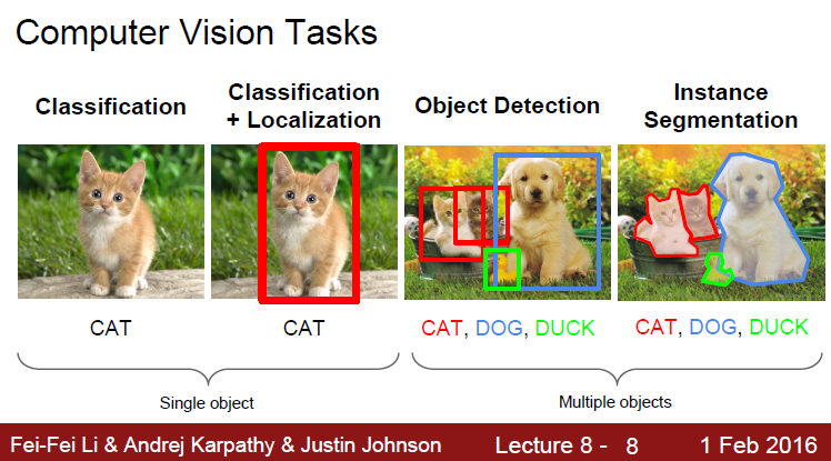
- Classification : 사진에 대한 라벨이 아웃풋
- Localization : 사진에 대한 상자가 아웃풋 (x, y, w, h)
- Detection : 사진에 대한 여러개의 상자가 아웃풋 DOG(x, y, w, h), CAT(x, y, w, h), ...
- Segmentation : 상자가 아니라 객체의 이미지 형상을 그대로.
-
Localization method : localization as Regression, Sliding Window : Overfeat
-
Region Proposals : 비슷한 색깔, 텍스쳐를 기준으로 박스를 생성
-
Detection :
- R-CNN : Region-based CNN. Region -> CNN
- 문제점 : Region proposal 마다 CNN을 돌려서 시간이 매우 많이든다.
- Fast R-CNN : CNN -> Region
- 문제점 : Region Proposal 과정에서 시간이 든다.
-
Faster R-CNN : Region Proposals도 CNN을 이용해서 해보자.
-
YOLO(You Only Look Once) : Detection as Regression
- 성능은 Faster R-CNN보다 떨어지지만, 속도가 매우 빠르다.
- R-CNN : Region-based CNN. Region -> CNN
-
Data Augmentation
- Change the pixels without changing the label
- Train on transformed data
-
VERY widely used
.....
- Horizontal flips
- Random crops/scales
- Color jitter
-
Transfer learning
이미지넷의 클래스와 관련있는 데이터라면 사전학습시 성능이 좋아지는게 이해가되는데 관련없는 이미지 (e.g. mri같은 의료이미지)의 경우도 성능이 좋아지는데 그 이유는 무엇인가?
-> 앞단에선 엣지, 컬러같은 low level의 feature를 인식, 뒤로갈수록 상위레벨을 인식. lowlevel을 미리 학습해놓는다는 것은 그 어떤 이미지를 분석할 때도 도움이된다!
-
How to stack convolutions:
- Replace large convolutions (5x5, 7x7) with stacks of 3x3 convolutions
- 1x1 "bottleneck" convolutions are very efficient
- Can factor NxN convolutions into 1xN and Nx1
-
All of the above give fewer parameters, less compute, more nonlinearity
더 적은 파라미터, 더 적은 컴퓨팅연산, 더 많은 nonlinearity(필터 사이사이 ReLU등이 들어가기에)
- Computing Convolutions:
- im2col : Easy to implement, but big memory overhead.
- FFT : Big speedups for small kernels
- "Fast Algorithms" : seem promising, not widely used yet
- Semantic Segmentation
- Classify all pixels
- Fully convolutional models, downsample then upsample
- Learnable upsampling: fractionally strided convolution
- Skip connections can help
...
- Instance Segmentation
- Detect instance, generate mask
- Similar pipelines to object detection